Excel Matrix Multiplication – Replacing MMULT with Power Query

In my last Thank You post, I suggested that Matrix multiplication is not Excel’s forte. Following that post, I got a cool Power Query solution from Imke Feldmann, author of ThedBIccountant.com, that performs matrix multiplication with Power Query.

So today I decided to share with you my version of a Matrix Multiplication using Power Query. I am looking forward to hear your comments.

Before we start, if you insist on using Excel for matrix multiplication, let’s explain why you should consider the Power Query option instead of the array formula MMULT in Excel.

MMULT function in Excel requires a manual selection of the new dimensions of the matrix A*B whenever one of your matrices A or B changes their dimensions.

For example, if A is a 3×2 matrix and B is a 2×4 matrix. A*B is should be a 3×4 matrix. (If you forgot the definition of matrix multiplication go here).

Now imagine that matrix A grows by one row, so it becomes a 4×2 matrix, which should make A*B a 4×4 matrix. As a result, if you use MMULT, you should manually select the a new range of the array function, and click the CTRL+Shift+Enter to invoke it.

Using MMULT can become a tedious and repetitive manual labor, if matrix A constantly expands with new rows, or matrix B expands with new columns. I don’t envy the data analysts that need to update their workbooks each time with the necessary error-prone manual steps.

Luckily for us, we have Power Query technology in Excel and Power BI, With Power Query you can automate your matrix multiplication without the need to perform manual adjustments whenever the dimensions change.

Download this workbook to see Power Query’s version for matrix multiplication in action.
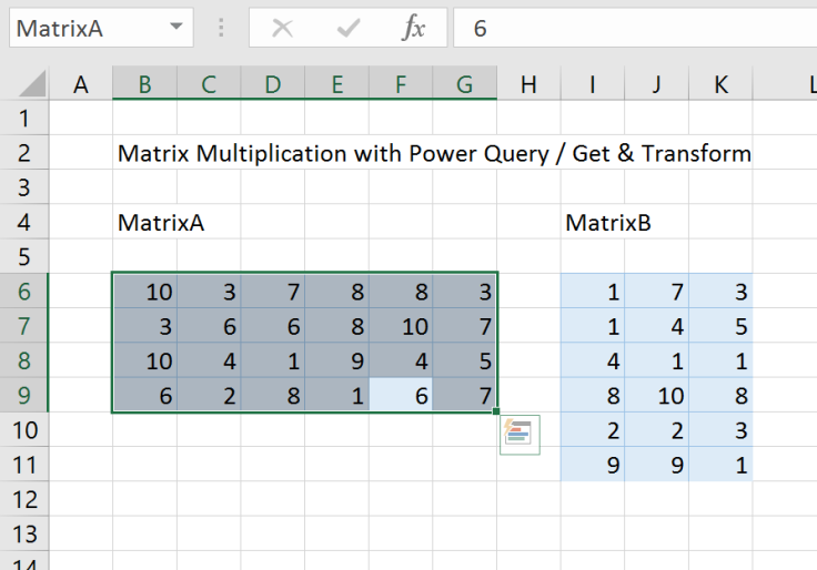
In this shared workbook we have matrix A and matrix B as two named ranges MatrixA and MatrixB. More specifically, the range B6:G9 is defined as the name range MatrixA, and the range I6:K11 os defined as MatrixB.

Now, using the Power Query M expression below, you can perform the matrix multiplication of A*B.

(In the shared workbook you get everything to start multiplying matrices, so if you are not a Power Query expert, you can skip this block of code).

let
 MatrixA = Excel.CurrentWorkbook(){[Name="MatrixA"]}[Content],
 MatrixB = Excel.CurrentWorkbook(){[Name="MatrixB"]}[Content],
 RowIndices = List.Numbers(0,Table.RowCount(MatrixA)),
 ColumnIndices = List.Numbers(0,Table.ColumnCount(MatrixB)),
 #"Converted to Table" = Table.FromList(
  RowIndices, Splitter.SplitByNothing(), null, null, ExtraValues.Error),
 #"Renamed Columns" = Table.RenameColumns(#"Converted to Table",
  {{"Column1", "Row"}}),
 #"Added Custom" = Table.AddColumn(#"Renamed Columns", "Custom",
  each ColumnIndices),
 #"Renamed Columns1" = Table.RenameColumns(#"Added Custom",
  {{"Custom", "Column"}}),
 #"Expanded Custom" = Table.ExpandListColumn(#"Renamed Columns1", "Column"),
 #"Added Custom1" = Table.AddColumn(#"Expanded Custom", "Row Data",
  each Record.FieldValues(MatrixA{[Row]})),
 MatrixBColumns = Table.ToColumns(MatrixB),
 #"Added Custom2" = Table.AddColumn(#"Added Custom1", "Column Data",
  each MatrixBColumns{[Column]}),
 
 fnMatrixProduct = (list1, list2) =>
  List.Sum(
   List.Generate(
    ()=>[A=list1,B=list2, Index=0],
    each [Index] < List.Count([A]),
    each [A=[A],B=[B],Index =[Index]+1],
    each [A]{[Index]}*[B]{[Index]}
   )
  ),

 #"Added Custom3" = Table.AddColumn(#"Added Custom2",
  "Custom", each fnMatrixProduct([Row Data],[Column Data])),
 #"Removed Columns" = Table.RemoveColumns(#"Added Custom3",
  {"Row Data", "Column Data"}),
 #"Pivoted Column" = Table.Pivot(Table.TransformColumnTypes(#"Removed Columns",
  {{"Column", type text}}, "en-US"),
  List.Distinct(Table.TransformColumnTypes(#"Removed Columns",
   {{"Column", type text}}, "en-US")[Column]), "Column", "Custom")
in
 #"Pivoted Column"

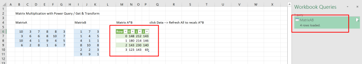
You can see the result which is the matrix A*B in the shared workbook. To refresh the calculation click Data–>Refresh All, or just refresh the query MatrixAB in the Workbook Queries pane.

Note: Whenever one of the matrices change by value or dimension, refreshing the workbook will load the result.

If you are an advanced Power Query user, and want to learn how the expression above works, please let me know.

In this post I will focus only on the core transformation which uses the function List.Generate to perform the main matrix multiplication calculation of an individual cell in the matrix A*B.

In the M expression above we use the function fnMatrixProduct, which uses List.Generate to iterate over a given row from A and a column from B and calculate the single cell in A*B.

 fnMatrixProduct = (list1, list2) =>
  List.Sum(
   List.Generate(()=>[A=list1,B=list2, Index=0],
    each [Index] < List.Count([A]),
    each [A=[A],B=[B],Index =[Index]+1],
    each [A]{[Index]}*[B]{[Index]})),

Since Power Query uses a functional language for the transformation it was not designed to perform loop iterations, well, at least not directly. So we are using List.Generate to iterate over the two input lists and generate a new list whose elements are the product of the elements in the input lists.

List.Generate function consists of 4 arguments (more here):

Argument	Description
start	A function that provides the initial value
condition	A condition which controls the sequence of generation
next	A function that generates the next value for an iteration
transfomer	A transformation function to apply to each item in the list

Let’s explain how we implemented each argument here:

List.Generate(
 ()=>[A=list1,B=list2, Index=0],
 each [Index] < List.Count([A]),
 each [A=[A],B=[B],Index =[Index]+1],
 each [A]{[Index]}*[B]{[Index]})
),

Part 1: The “start” argument

()=>[A=list1,B=list2, Index=0],

This argument contains the record (a Key-Value pairs which are used to define the state during the list generation). The record is used as the starting state for our loop, and can be accessed and modified at each iteration step. We assign the key A with the value of list1, and key B with list2. The last field in the record is used for the running index.

Part 2: The “condition” argument

each [Index] < List.Count([A]),

This part contains the condition that should be met in each iteration. When the conditon is not met, the generation of the new list stops. Since Index starts with zero, we should stop generating the list when Index equal to one of the lists’ size.

Part 3: The “next” argument

each [A=[A],B=[B],Index =[Index]+1],

This argument defines the changes we should perform on record, before the next iteration. In our case, we keep the keys A and B with the original input lists, and increment the index by 1.

Part 4: The “transformer” argument

 each [A]{[Index]}*[B]{[Index]})

This argument contains the main calculation step. It defines the arithmetic operation we perform when we generate the k’th element in the new list. We read the k’th values in each list and multiply them. The result is stored as a new element in the list.

The output of List.Generate is a list of products. Now we just need to apply the ∑ part of the formula above, and for that we can use function List.Sum.

fnMatrixProduct = (list1, list2) =>
  List.Sum(
   List.Generate(...),

That’s it for today. On my next blog post I may go further and explain the rest of the query. But no promises 🙂

Io conclude this blog post, I will be glad to hear your feedback and learn more about your scenarios for using matrix multiplication in Excel. I am sure that the new technique is much better than the classic MMULT array formula.

Update: 6/6/2016: It turns out that the query above is relatively slow. I got faster versions from Bill Szysz, and Imke Feldmann. I have updated the faster query here, and a new blog post here with the step-by-step instructions.

Enjoy,

Gil